18 Expressions
18.1 Introduction
To compute on the language, we first need to understand its structure. That requires some new vocabulary, some new tools, and some new ways of thinking about R code. The first of these is the distinction between an operation and its result. Take the following code, which multiplies a variable x by 10 and saves the result to a new variable called y. It doesn’t work because we haven’t defined a variable called x:
y <- x * 10
#> Error: object 'x' not found
It would be nice if we could capture the intent of the code without executing it. In other words, how can we separate our description of the action from the action itself?
One way is to use rlang::expr():
z <- rlang::expr(y <- x * 10)
z
#> y <- x * 10
expr() returns an expression, an object that captures the structure of the code without evaluating it (i.e. running it). If you have an expression, you can evaluate it with base::eval():
x <- 4
eval(z)
y
#> [1] 40
The focus of this chapter is the data structures that underlie expressions. Mastering this knowledge will allow you to inspect and modify captured code, and to generate code with code. We’ll come back to expr() in Chapter 19, and to eval() in Chapter 20.
Outline
Section 18.2 introduces the idea of the abstract syntax tree (AST), and reveals the tree like structure that underlies all R code.
Section 18.3 dives into the details of the data structures that underpin the AST: constants, symbols, and calls, which are collectively known as expressions.
Section 18.4 covers parsing, the act of converting the linear sequence of character in code into the AST, and uses that idea to explore some details of R’s grammar.
Section 18.5 shows you how you can use recursive functions to compute on the language, writing functions that compute with expressions.
Section 18.6 circles back to three more specialised data structures: pairlists, missing arguments, and expression vectors.
18.2 Abstract syntax trees
Expressions are also called abstract syntax trees (ASTs) because the structure of code is hierarchical and can be naturally represented as a tree. Understanding this tree structure is crucial for inspecting and modifying expressions (i.e. metaprogramming).
18.2.1 Drawing
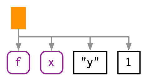
We’ll start by introducing some conventions for drawing ASTs, beginning with a simple call that shows their main components: f(x, "y", 1). I’ll draw trees in two ways89:
-
By “hand” (i.e. with OmniGraffle):
-
With
lobstr::ast():lobstr::ast(f(x, "y", 1)) #> █─f #> ├─x #> ├─"y" #> └─1
Both approaches share conventions as much as possible:
The leaves of the tree are either symbols, like
fandx, or constants, like1or"y". Symbols are drawn in purple and have rounded corners. Constants have black borders and square corners. Strings and symbols are easily confused, so strings are always surrounded in quotes.The branches of the tree are call objects, which represent function calls, and are drawn as orange rectangles. The first child (
f) is the function that gets called; the second and subsequent children (x,"y", and1) are the arguments to that function.
Colours will be shown when you call ast(), but do not appear in the book for complicated technical reasons.
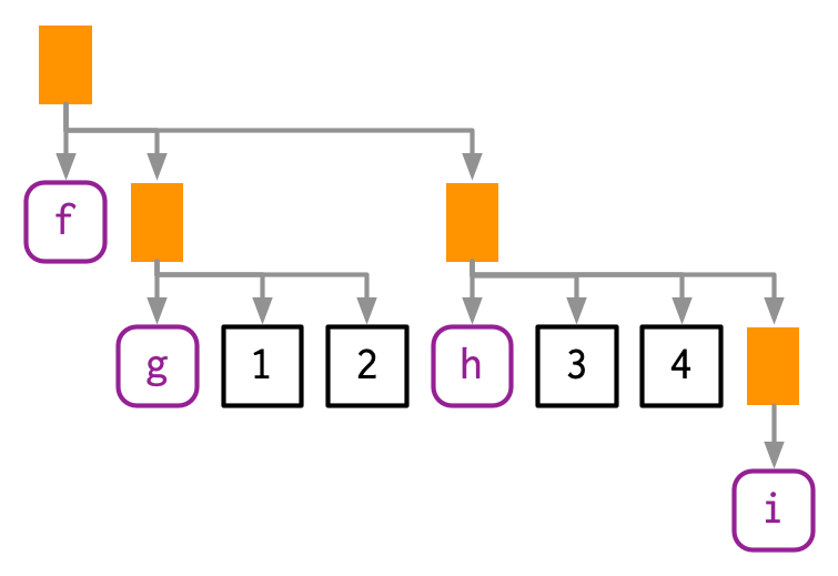
The above example only contained one function call, making for a very shallow tree. Most expressions will contain considerably more calls, creating trees with multiple levels. For example, consider the AST for f(g(1, 2), h(3, 4, i())):
lobstr::ast(f(g(1, 2), h(3, 4, i())))
#> █─f
#> ├─█─g
#> │ ├─1
#> │ └─2
#> └─█─h
#>   ├─3
#>   ├─4
#>   └─█─i
You can read the hand-drawn diagrams from left-to-right (ignoring vertical position), and the lobstr-drawn diagrams from top-to-bottom (ignoring horizontal position). The depth within the tree is determined by the nesting of function calls. This also determines evaluation order, as evaluation generally proceeds from deepest-to-shallowest, but this is not guaranteed because of lazy evaluation (Section 6.5). Also note the appearance of i(), a function call with no arguments; it’s a branch with a single (symbol) leaf.
18.2.2 Non-code components
You might have wondered what makes these abstract syntax trees. They are abstract because they only capture important structural details of the code, not whitespace or comments:
ast(
  f(x,  y)  # important!
)
#> █─f
#> ├─x
#> └─y
There’s only one place where whitespace affects the AST:
18.2.3 Infix calls
Every call in R can be written in tree form because any call can be written in prefix form (Section 6.8.1). Take y <- x * 10 again: what are the functions that are being called? It is not as easy to spot as f(x, 1) because this expression contains two infix calls: <- and *. That means that these two lines of code are equivalent:
y <- x * 10
`<-`(y, `*`(x, 10))
And they both have this AST90:
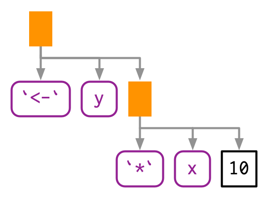
lobstr::ast(y <- x * 10)
#> █─`<-`
#> ├─y
#> └─█─`*`
#>   ├─x
#>   └─10
There really is no difference between the ASTs, and if you generate an expression with prefix calls, R will still print it in infix form:
expr(`<-`(y, `*`(x, 10)))
#> y <- x * 10
The order in which infix operators are applied is governed by a set of rules called operator precedence, and we’ll use lobstr::ast() to explore them in Section 18.4.1.
18.2.4 Exercises
-
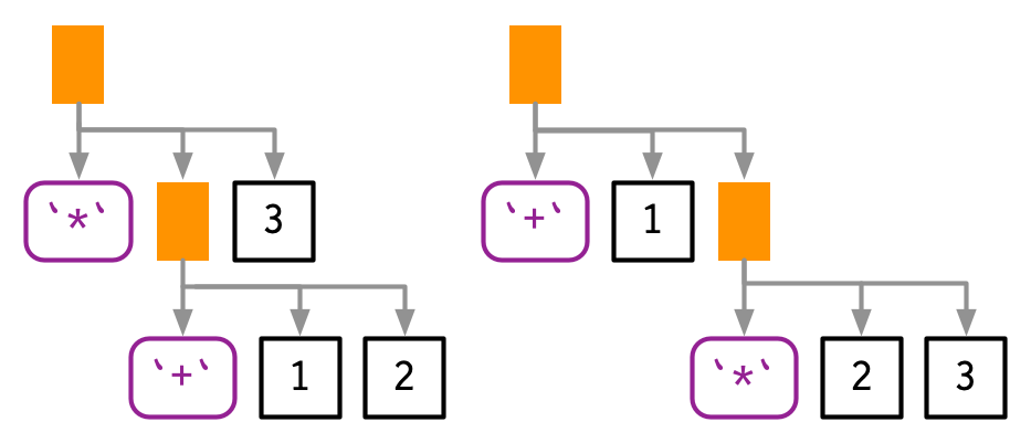
Reconstruct the code represented by the trees below:
#> █─f #> └─█─g #> └─█─h #> █─`+` #> ├─█─`+` #> │ ├─1 #> │ └─2 #> └─3 #> █─`*` #> ├─█─`(` #> │ └─█─`+` #> │ ├─x #> │ └─y #> └─z -
Draw the following trees by hand and then check your answers with
lobstr::ast().f(g(h(i(1, 2, 3)))) f(1, g(2, h(3, i()))) f(g(1, 2), h(3, i(4, 5))) -
What’s happening with the ASTs below? (Hint: carefully read
?"^".) -
What is special about the AST below? (Hint: re-read Section 6.2.1.)
lobstr::ast(function(x = 1, y = 2) {})
#> █─`function`
#> ├─█─x = 1
#> │ └─y = 2
#> ├─█─`{`
#> └─NULL
What does the call tree of an
ifstatement with multipleelse ifconditions look like? Why?
18.3 Expressions
Collectively, the data structures present in the AST are called expressions. An expression is any member of the set of base types created by parsing code: constant scalars, symbols, call objects, and pairlists. These are the data structures used to represent captured code from expr(), and is_expression(expr(...)) is always true91. Constants, symbols and call objects are the most important, and are discussed below. Pairlists and empty symbols are more specialised and we’ll come back to them in Sections 18.6.1 and Section 18.6.2.
NB: In base R documentation “expression” is used to mean two things. As well as the definition above, expression is also used to refer to the type of object returned by expression() and parse(), which are basically lists of expressions as defined above. In this book I’ll call these expression vectors, and I’ll come back to them in Section 18.6.3.
18.3.1 Constants
Scalar constants are the simplest component of the AST. More precisely, a constant is either NULL or a length-1 atomic vector (or scalar, Section 3.2.1) like TRUE, 1L, 2.5 or "x". You can test for a constant with rlang::is_syntactic_literal().
Constants are self-quoting in the sense that the expression used to represent a constant is the same constant:
18.3.2 Symbols
A symbol represents the name of an object like x, mtcars, or mean. In base R, the terms symbol and name are used interchangeably (i.e. is.name() is identical to is.symbol()), but in this book I used symbol consistently because “name” has many other meanings.
You can create a symbol in two ways: by capturing code that references an object with expr(), or turning a string into a symbol with rlang::sym():
You can turn a symbol back into a string with as.character() or rlang::as_string(). as_string() has the advantage of clearly signalling that you’ll get a character vector of length 1.
You can recognise a symbol because it’s printed without quotes, str() tells you that it’s a symbol, and is.symbol() is TRUE:
The symbol type is not vectorised, i.e. a symbol is always length 1. If you want multiple symbols, you’ll need to put them in a list, using (e.g.) rlang::syms().
18.3.3 Calls
A call object represents a captured function call. Call objects are a special type of list92 where the first component specifies the function to call (usually a symbol), and the remaining elements are the arguments for that call. Call objects create branches in the AST, because calls can be nested inside other calls.
You can identify a call object when printed because it looks just like a function call. Confusingly typeof() and str() print “language”93 for call objects, but is.call() returns TRUE:
lobstr::ast(read.table("important.csv", row.names = FALSE))
#> █─read.table
#> ├─"important.csv"
#> └─row.names = FALSE
x <- expr(read.table("important.csv", row.names = FALSE))

typeof(x)
#> [1] "language"
is.call(x)
#> [1] TRUE
18.3.3.1 Subsetting
Calls generally behave like lists, i.e. you can use standard subsetting tools. The first element of the call object is the function to call, which is usually a symbol:
x[[1]]
#> read.table
is.symbol(x[[1]])
#> [1] TRUE
The remainder of the elements are the arguments:
as.list(x[-1])
#> [[1]]
#> [1] "important.csv"
#>
#> $row.names
#> [1] FALSE
You can extract individual arguments with [[ or, if named, $:
x[[2]]
#> [1] "important.csv"
x$row.names
#> [1] FALSE
You can determine the number of arguments in a call object by subtracting 1 from its length:
length(x) - 1
#> [1] 2
Extracting specific arguments from calls is challenging because of R’s flexible rules for argument matching: it could potentially be in any location, with the full name, with an abbreviated name, or with no name. To work around this problem, you can use rlang::call_standardise() which standardises all arguments to use the full name:
rlang::call_standardise(x)
#> Warning: `call_standardise()` is deprecated as of rlang 0.4.11
#> This warning is displayed once every 8 hours.
#> read.table(file = "important.csv", row.names = FALSE)
(NB: If the function uses ... it’s not possible to standardise all arguments.)
Calls can be modified in the same way as lists:
x$header <- TRUE
x
#> read.table("important.csv", row.names = FALSE, header = TRUE)
18.3.3.2 Function position
The first element of the call object is the function position. This contains the function that will be called when the object is evaluated, and is usually a symbol94:
lobstr::ast(foo())
#> █─foo
While R allows you to surround the name of the function with quotes, the parser converts it to a symbol:
lobstr::ast("foo"())
#> █─foo
However, sometimes the function doesn’t exist in the current environment and you need to do some computation to retrieve it: for example, if the function is in another package, is a method of an R6 object, or is created by a function factory. In this case, the function position will be occupied by another call:
lobstr::ast(pkg::foo(1))
#> █─█─`::`
#> │ ├─pkg
#> │ └─foo
#> └─1
lobstr::ast(obj$foo(1))
#> █─█─`$`
#> │ ├─obj
#> │ └─foo
#> └─1
lobstr::ast(foo(1)(2))
#> █─█─foo
#> │ └─1
#> └─2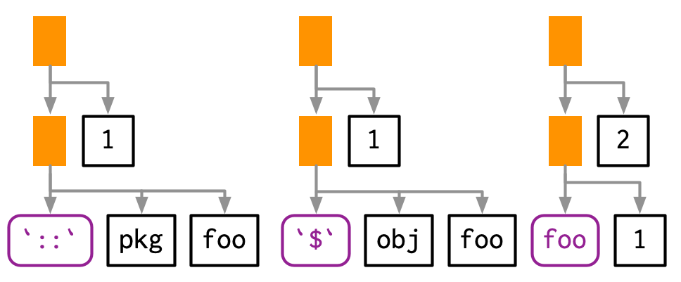
18.3.3.3 Constructing
You can construct a call object from its components using rlang::call2(). The first argument is the name of the function to call (either as a string, a symbol, or another call). The remaining arguments will be passed along to the call:
call2("mean", x = expr(x), na.rm = TRUE)
#> mean(x = x, na.rm = TRUE)
call2(expr(base::mean), x = expr(x), na.rm = TRUE)
#> base::mean(x = x, na.rm = TRUE)
Infix calls created in this way still print as usual.
Using call2() to create complex expressions is a bit clunky. You’ll learn another technique in Chapter 19.
18.3.4 Summary
The following table summarises the appearance of the different expression subtypes in str() and typeof():
str() |
typeof() |
|
|---|---|---|
| Scalar constant |
logi/int/num/chr
|
logical/integer/double/character
|
| Symbol | symbol |
symbol |
| Call object | language |
language |
| Pairlist | Dotted pair list | pairlist |
| Expression vector | expression() |
expression |
Both base R and rlang provide functions for testing for each type of input, although the types covered are slightly different. You can easily tell them apart because all the base functions start with is. and the rlang functions start with is_.
| base | rlang | |
|---|---|---|
| Scalar constant | — | is_syntactic_literal() |
| Symbol | is.symbol() |
is_symbol() |
| Call object | is.call() |
is_call() |
| Pairlist | is.pairlist() |
is_pairlist() |
| Expression vector | is.expression() |
— |
18.3.5 Exercises
Which two of the six types of atomic vector can’t appear in an expression? Why? Similarly, why can’t you create an expression that contains an atomic vector of length greater than one?
What happens when you subset a call object to remove the first element? e.g.
expr(read.csv("foo.csv", header = TRUE))[-1]. Why?-
Describe the differences between the following call objects.
-
rlang::call_standardise()doesn’t work so well for the following calls. Why? What makesmean()special?call_standardise(quote(mean(1:10, na.rm = TRUE))) #> mean(x = 1:10, na.rm = TRUE) call_standardise(quote(mean(n = T, 1:10))) #> mean(x = 1:10, n = T) call_standardise(quote(mean(x = 1:10, , TRUE))) #> mean(x = 1:10, , TRUE) -
Why does this code not make sense?
Construct the expression
if(x > 1) "a" else "b"using multiple calls tocall2(). How does the code structure reflect the structure of the AST?
18.4 Parsing and grammar
We’ve talked a lot about expressions and the AST, but not about how expressions are created from code that you type (like "x + y"). The process by which a computer language takes a string and constructs an expression is called parsing, and is governed by a set of rules known as a grammar. In this section, we’ll use lobstr::ast() to explore some of the details of R’s grammar, and then show how you can transform back and forth between expressions and strings.
18.4.1 Operator precedence
Infix functions introduce two sources of ambiguity95. The first source of ambiguity arises from infix functions: what does 1 + 2 * 3 yield? Do you get 9 (i.e. (1 + 2) * 3), or 7 (i.e. 1 + (2 * 3))? In other words, which of the two possible parse trees below does R use?
Programming languages use conventions called operator precedence to resolve this ambiguity. We can use ast() to see what R does:
lobstr::ast(1 + 2 * 3)
#> █─`+`
#> ├─1
#> └─█─`*`
#>   ├─2
#>   └─3
Predicting the precedence of arithmetic operations is usually easy because it’s drilled into you in school and is consistent across the vast majority of programming languages.
Predicting the precedence of other operators is harder. There’s one particularly surprising case in R: ! has a much lower precedence (i.e. it binds less tightly) than you might expect. This allows you to write useful operations like:
R has over 30 infix operators divided into 18 precedence groups. While the details are described in ?Syntax, very few people have memorised the complete ordering. If there’s any confusion, use parentheses!
lobstr::ast((1 + 2) * 3)
#> █─`*`
#> ├─█─`(`
#> │ └─█─`+`
#> │   ├─1
#> │   └─2
#> └─3
Note the appearance of the parentheses in the AST as a call to the ( function.
18.4.2 Associativity
The second source of ambiguity is introduced by repeated usage of the same infix function. For example, is 1 + 2 + 3 equivalent to (1 + 2) + 3 or to 1 + (2 + 3)? This normally doesn’t matter because x + (y + z) == (x + y) + z, i.e. addition is associative, but is needed because some S3 classes define + in a non-associative way. For example, ggplot2 overloads + to build up a complex plot from simple pieces; this is non-associative because earlier layers are drawn underneath later layers (i.e. geom_point() + geom_smooth() does not yield the same plot as geom_smooth() + geom_point()).
In R, most operators are left-associative, i.e. the operations on the left are evaluated first:
lobstr::ast(1 + 2 + 3)
#> █─`+`
#> ├─█─`+`
#> │ ├─1
#> │ └─2
#> └─3
There are two exceptions: exponentiation and assignment.
18.4.3 Parsing and deparsing
Most of the time you type code into the console, and R takes care of turning the characters you’ve typed into an AST. But occasionally you have code stored in a string, and you want to parse it yourself. You can do so using rlang::parse_expr():
x1 <- "y <- x + 10"
x1
#> [1] "y <- x + 10"
is.call(x1)
#> [1] FALSE

x2 <- rlang::parse_expr(x1)
x2
#> y <- x + 10
is.call(x2)
#> [1] TRUE
parse_expr() always returns a single expression. If you have multiple expression separated by ; or \n, you’ll need to use rlang::parse_exprs(). It returns a list of expressions:
x3 <- "a <- 1; a + 1"
rlang::parse_exprs(x3)
#> [[1]]
#> a <- 1
#>
#> [[2]]
#> a + 1
If you find yourself working with strings containing code very frequently, you should reconsider your process. Read Chapter 19 and consider whether you can generate expressions using quasiquotation more safely.
The base equivalent to parse_exprs() is parse(). It is a little harder to use because it’s specialised for parsing R code stored in files. You need to supply your string to the text argument and it returns an expression vector (Section 18.6.3). I recommend turning the output into a list:
The inverse of parsing is deparsing: given an expression, you want the string that would generate it. This happens automatically when you print an expression, and you can get the string with rlang::expr_text():
Parsing and deparsing are not perfectly symmetric because parsing generates an abstract syntax tree. This means we lose backticks around ordinary names, comments, and whitespace:
Be careful when using the base R equivalent, deparse(): it returns a character vector with one element for each line. Whenever you use it, remember that the length of the output might be greater than one, and plan accordingly.
18.4.4 Exercises
-
R uses parentheses in two slightly different ways as illustrated by these two calls:
f((1))
`(`(1 + 1)
Compare and contrast the two uses by referencing the AST.
=can also be used in two ways. Construct a simple example that shows both uses.Does
-2^2yield 4 or -4? Why?What does
!1 + !1return? Why?Why does
x1 <- x2 <- x3 <- 0work? Describe the two reasons.Compare the ASTs of
x + y %+% zandx ^ y %+% z. What have you learned about the precedence of custom infix functions?What happens if you call
parse_expr()with a string that generates multiple expressions? e.g.parse_expr("x + 1; y + 1")What happens if you attempt to parse an invalid expression? e.g.
"a +"or"f())".-
deparse()produces vectors when the input is long. For example, the following call produces a vector of length two:expr <- expr(g(a + b + c + d + e + f + g + h + i + j + k + l + m + n + o + p + q + r + s + t + u + v + w + x + y + z)) deparse(expr)What does
expr_text()do instead? pairwise.t.test()assumes thatdeparse()always returns a length one character vector. Can you construct an input that violates this expectation? What happens?
18.5 Walking AST with recursive functions
To conclude the chapter I’m going to use everything you’ve learned about ASTs to solve more complicated problems. The inspiration comes from the base codetools package, which provides two interesting functions:
findGlobals()locates all global variables used by a function. This can be useful if you want to check that your function doesn’t inadvertently rely on variables defined in their parent environment.checkUsage()checks for a range of common problems including unused local variables, unused parameters, and the use of partial argument matching.
Getting all of the details of these functions correct is fiddly, so we won’t fully develop the ideas. Instead we’ll focus on the big underlying idea: recursion on the AST. Recursive functions are a natural fit to tree-like data structures because a recursive function is made up of two parts that correspond to the two parts of the tree:
The recursive case handles the nodes in the tree. Typically, you’ll do something to each child of a node, usually calling the recursive function again, and then combine the results back together again. For expressions, you’ll need to handle calls and pairlists (function arguments).
The base case handles the leaves of the tree. The base cases ensure that the function eventually terminates, by solving the simplest cases directly. For expressions, you need to handle symbols and constants in the base case.
To make this pattern easier to see, we’ll need two helper functions. First we define expr_type() which will return “constant” for constant, “symbol” for symbols, “call”, for calls, “pairlist” for pairlists, and the “type” of anything else:
expr_type <- function(x) {
  if (rlang::is_syntactic_literal(x)) {
    "constant"
  } else if (is.symbol(x)) {
    "symbol"
  } else if (is.call(x)) {
    "call"
  } else if (is.pairlist(x)) {
    "pairlist"
  } else {
    typeof(x)
  }
}

expr_type(expr("a"))
#> [1] "constant"
expr_type(expr(x))
#> [1] "symbol"
expr_type(expr(f(1, 2)))
#> [1] "call"
We’ll couple this with a wrapper around the switch function:
switch_expr <- function(x, ...) {
  switch(expr_type(x),
    ...,
    stop("Don't know how to handle type ", typeof(x), call. = FALSE)
  )
}
With these two functions in hand, we can write a basic template for any function that walks the AST using switch() (Section 5.2.3):
recurse_call <- function(x) {
  switch_expr(x,
    # Base cases
    symbol = ,
    constant = ,

    # Recursive cases
    call = ,
    pairlist =
  )
}
Typically, solving the base case is easy, so we’ll do that first, then check the results. The recursive cases are trickier, and will often require some functional programming.
18.5.1 Finding F and T
We’ll start with a function that determines whether another function uses the logical abbreviations T and F because using them is often considered to be poor coding practice. Our goal is to return TRUE if the input contains a logical abbreviation, and FALSE otherwise.
Let’s first find the type of T versus TRUE:
TRUE is parsed as a logical vector of length one, while T is parsed as a name. This tells us how to write our base cases for the recursive function: a constant is never a logical abbreviation, and a symbol is an abbreviation if it’s “F” or “T”:
logical_abbr_rec <- function(x) {
  switch_expr(x,
    constant = FALSE,
    symbol = as_string(x) %in% c("F", "T")
  )
}

logical_abbr_rec(expr(TRUE))
#> [1] FALSE
logical_abbr_rec(expr(T))
#> [1] TRUE
I’ve written logical_abbr_rec() function assuming that the input will be an expression as this will make the recursive operation simpler. However, when writing a recursive function it’s common to write a wrapper that provides defaults or makes the function a little easier to use. Here we’ll typically make a wrapper that quotes its input (we’ll learn more about that in the next chapter), so we don’t need to use expr() every time.
logical_abbr <- function(x) {
  logical_abbr_rec(enexpr(x))
}

logical_abbr(T)
#> [1] TRUE
logical_abbr(FALSE)
#> [1] FALSE
Next we need to implement the recursive cases. Here we want to do the same thing for calls and for pairlists: recursively apply the function to each subcomponent, and return TRUE if any subcomponent contains a logical abbreviation. This is made easy by purrr::some(), which iterates over a list and returns TRUE if the predicate function is true for any element.
18.5.2 Finding all variables created by assignment
logical_abbr() is relatively simple: it only returns a single TRUE or FALSE. The next task, listing all variables created by assignment, is a little more complicated. We’ll start simply, and then make the function progressively more rigorous.
We start by looking at the AST for assignment:
ast(x <- 10)
#> █─`<-`
#> ├─x
#> └─10
Assignment is a call object where the first element is the symbol <-, the second is the name of variable, and the third is the value to be assigned.
Next, we need to decide what data structure we’re going to use for the results. Here I think it will be easiest if we return a character vector. If we return symbols, we’ll need to use a list() and that makes things a little more complicated.
With that in hand we can start by implementing the base cases and providing a helpful wrapper around the recursive function. Here the base cases are straightforward because we know that neither a symbol nor a constant represents assignment.
find_assign_rec <- function(x) {
  switch_expr(x,
    constant = ,
    symbol = character()
  )
}
find_assign <- function(x) find_assign_rec(enexpr(x))

find_assign("x")
#> character(0)
find_assign(x)
#> character(0)
Next we implement the recursive cases. This is made easier by a function that should exist in purrr, but currently doesn’t. flat_map_chr() expects .f to return a character vector of arbitrary length, and flattens all results into a single character vector.
flat_map_chr <- function(.x, .f, ...) {
  purrr::flatten_chr(purrr::map(.x, .f, ...))
}

flat_map_chr(letters[1:3], ~ rep(., sample(3, 1)))
#> [1] "a" "b" "b" "b" "c" "c" "c"
The recursive case for pairlists is straightforward: we iterate over every element of the pairlist (i.e. each function argument) and combine the results. The case for calls is a little bit more complex: if this is a call to <- then we should return the second element of the call:
find_assign_rec <- function(x) {
  switch_expr(x,
    # Base cases
    constant = ,
    symbol = character(),

    # Recursive cases
    pairlist = flat_map_chr(as.list(x), find_assign_rec),
    call = {
      if (is_call(x, "<-")) {
        as_string(x[[2]])
      } else {
        flat_map_chr(as.list(x), find_assign_rec)
      }
    }
  )
}

find_assign(a <- 1)
#> [1] "a"
find_assign({
  a <- 1
  {
    b <- 2
  }
})
#> [1] "a" "b"
Now we need to make our function more robust by coming up with examples intended to break it. What happens when we assign to the same variable multiple times?
find_assign({
  a <- 1
  a <- 2
})
#> [1] "a" "a"
It’s easiest to fix this at the level of the wrapper function:
find_assign <- function(x) unique(find_assign_rec(enexpr(x)))

find_assign({
  a <- 1
  a <- 2
})
#> [1] "a"
What happens if we have nested calls to <-? Currently we only return the first. That’s because when <- occurs we immediately terminate recursion.
find_assign({
  a <- b <- c <- 1
})
#> [1] "a"
Instead we need to take a more rigorous approach. I think it’s best to keep the recursive function focused on the tree structure, so I’m going to extract out find_assign_call() into a separate function.
find_assign_call <- function(x) {
  if (is_call(x, "<-") && is_symbol(x[[2]])) {
    lhs <- as_string(x[[2]])
    children <- as.list(x)[-1]
  } else {
    lhs <- character()
    children <- as.list(x)
  }

  c(lhs, flat_map_chr(children, find_assign_rec))
}

find_assign_rec <- function(x) {
  switch_expr(x,
    # Base cases
    constant = ,
    symbol = character(),

    # Recursive cases
    pairlist = flat_map_chr(x, find_assign_rec),
    call = find_assign_call(x)
  )
}

find_assign(a <- b <- c <- 1)
#> [1] "a" "b" "c"
find_assign(system.time(x <- print(y <- 5)))
#> [1] "x" "y"
The complete version of this function is quite complicated, it’s important to remember we wrote it by working our way up by writing simple component parts.
18.5.3 Exercises
logical_abbr()returnsTRUEforT(1, 2, 3). How could you modifylogical_abbr_rec()so that it ignores function calls that useTorF?-
logical_abbr()works with expressions. It currently fails when you give it a function. Why? How could you modifylogical_abbr()to make it work? What components of a function will you need to recurse over?logical_abbr(function(x = TRUE) { g(x + T) }) Modify
find_assignto also detect assignment using replacement functions, i.e.names(x) <- y.Write a function that extracts all calls to a specified function.
18.6 Specialised data structures
There are two data structures and one special symbol that we need to cover for the sake of completeness. They are not usually important in practice.
18.6.1 Pairlists
Pairlists are a remnant of R’s past and have been replaced by lists almost everywhere. The only place you are likely to see pairlists in R96 is when working with calls to the function function, as the formal arguments to a function are stored in a pairlist:
f <- expr(function(x, y = 10) x + y)

args <- f[[2]]
args
#> $x
#>
#>
#> $y
#> [1] 10
typeof(args)
#> [1] "pairlist"
Fortunately, whenever you encounter a pairlist, you can treat it just like a regular list:
Behind the scenes pairlists are implemented using a different data structure, a linked list instead of an array. That makes subsetting a pairlist much slower than subsetting a list, but this has little practical impact.
18.6.2 Missing arguments
The special symbol that needs a little extra discussion is the empty symbol, which is used to represent missing arguments (not missing values!). You only need to care about the missing symbol if you’re programmatically creating functions with missing arguments; we’ll come back to that in Section 19.4.3.
You can make an empty symbol with missing_arg() (or expr()):
missing_arg()
typeof(missing_arg())
#> [1] "symbol"
An empty symbol doesn’t print anything, so you can check if you have one with rlang::is_missing():
is_missing(missing_arg())
#> [1] TRUE
You’ll find them in the wild in function formals:
f <- expr(function(x, y = 10) x + y)
args <- f[[2]]
is_missing(args[[1]])
#> [1] TRUE
This is particularly important for ... which is always associated with an empty symbol:
f <- expr(function(...) list(...))
args <- f[[2]]
is_missing(args[[1]])
#> [1] TRUE
The empty symbol has a peculiar property: if you bind it to a variable, then access that variable, you will get an error:
m <- missing_arg()
m
#> Error: argument "m" is missing, with no default
But you won’t if you store it inside another data structure!
ms <- list(missing_arg(), missing_arg())
ms[[1]]
If you need to preserve the missingness of a variable, rlang::maybe_missing() is often helpful. It allows you to refer to a potentially missing variable without triggering the error. See the documentation for use cases and more details.
18.6.3 Expression vectors
Finally, we need to briefly discuss the expression vector. Expression vectors are only produced by two base functions: expression() and parse():
exp1 <- parse(text = c("
x <- 4
x
"))
exp2 <- expression(x <- 4, x)

typeof(exp1)
#> [1] "expression"
typeof(exp2)
#> [1] "expression"

exp1
#> expression(x <- 4, x)
exp2
#> expression(x <- 4, x)
Like calls and pairlists, expression vectors behave like lists:
length(exp1)
#> [1] 2
exp1[[1]]
#> x <- 4
Conceptually, an expression vector is just a list of expressions. The only difference is that calling eval() on an expression evaluates each individual expression. I don’t believe this advantage merits introducing a new data structure, so instead of expression vectors I just use lists of expressions.