16 Trade-offs
16.1 Introduction
You now know about the three most important OOP toolkits available in R. Now that you understand their basic operation and the principles that underlie them, we can start to compare and contrast the systems in order to understand their strengths and weaknesses. This will help you pick the system that is most likely to solve new problems.
Overall, when picking an OO system, I recommend that you default to S3. S3 is simple, and widely used throughout base R and CRAN. While it’s far from perfect, its idiosyncrasies are well understood and there are known approaches to overcome most shortcomings. If you have an existing background in programming you are likely to lean towards R6, because it will feel familiar. I think you should resist this tendency for two reasons. Firstly, if you use R6 it’s very easy to create a non-idiomatic API that will feel very odd to native R users, and will have surprising pain points because of the reference semantics. Secondly, if you stick to R6, you’ll lose out on learning a new way of thinking about OOP that gives you a new set of tools for solving problems.
Outline
Section 16.2 compares S3 and S4. In brief, S4 is more formal and tends to require more upfront planning. That makes it more suitable for big projects developed by teams, not individuals.
Section 16.3 compares S3 and R6. This section is quite long because these two systems are fundamentally different and there are a number of tradeoffs that you need to consider.
16.2 S4 versus S3
Once you’ve mastered S3, S4 is not too difficult to pick up: the underlying ideas are the same, S4 is just more formal, more strict, and more verbose. The strictness and formality of S4 make it well suited for large teams. Since more structure is provided by the system itself, there is less need for convention, and new contributors don’t need as much training. S4 tends to require more upfront design than S3, and this investment is more likely to pay off on larger projects where greater resources are available.
One large team effort where S4 is used to good effect is Bioconductor. Bioconductor is similar to CRAN: it’s a way of sharing packages amongst a wider audience. Bioconductor is smaller than CRAN (~1,300 versus ~10,000 packages, July 2017) and the packages tend to be more tightly integrated because of the shared domain and because Bioconductor has a stricter review process. Bioconductor packages are not required to use S4, but most will because the key data structures (e.g. SummarizedExperiment, IRanges, DNAStringSet) are built using S4.
S4 is also a good fit for complex systems of interrelated objects, and it’s possible to minimise code duplication through careful implementation of methods. The best example of such a system is the Matrix package.84 It is designed to efficiently store and compute with many different types of sparse and dense matrices. As of version 1.7.2, it defines 108 classes, 23 generic functions, and 1780 methods, and to give you some idea of the complexity, a small subset of the class graph is shown in Figure 16.1.
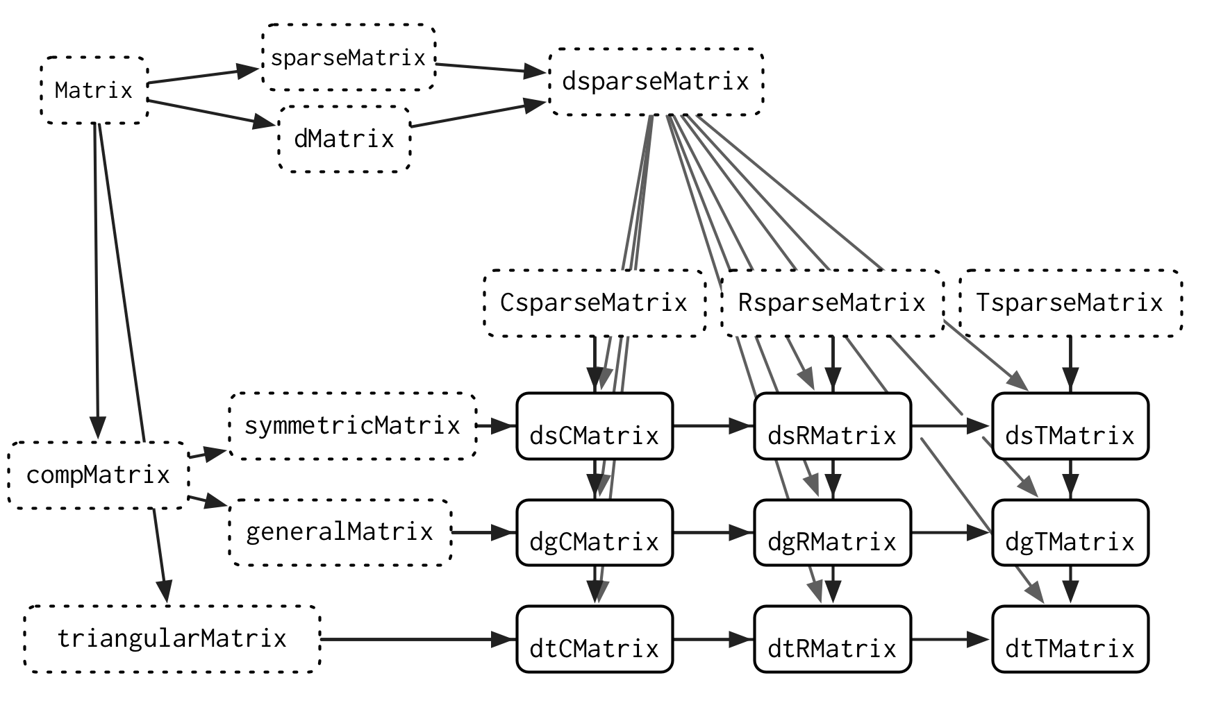
Figure 16.1: A small subset of the Matrix class graph showing the inheritance of sparse matrices. Each concrete class inherits from two virtual parents: one that describes how the data is stored (C = column oriented, R = row oriented, T = tagged) and one that describes any restriction on the matrix (s = symmetric, t = triangle, g = general).
This domain is a good fit for S4 because there are often computational shortcuts for specific combinations of sparse matrices. S4 makes it easy to provide a general method that works for all inputs, and then provide more specialised methods where the inputs allow a more efficient implementation. This requires careful planning to avoid method dispatch ambiguity, but the planning pays off with higher performance.
The biggest challenge to using S4 is the combination of increased complexity and absence of a single source of documentation. S4 is a complex system and it can be challenging to use effectively in practice. This wouldn’t be such a problem if S4 documentation wasn’t scattered through R documentation, books, and websites. S4 needs a book length treatment, but that book does not (yet) exist. (The documentation for S3 is no better, but the lack is less painful because S3 is much simpler.)
16.3 R6 versus S3
R6 is a profoundly different OO system from S3 and S4 because it is built on encapsulated objects, rather than generic functions. Additionally R6 objects have reference semantics, which means that they can be modified in place. These two big differences have a number of non-obvious consequences which we’ll explore here:
A generic is a regular function so it lives in the global namespace. An R6 method belongs to an object so it lives in a local namespace. This influences how we think about naming.
R6’s reference semantics allow methods to simultaneously return a value and modify an object. This solves a painful problem called “threading state”.
You invoke an R6 method using
$, which is an infix operator. If you set up your methods correctly you can use chains of method calls as an alternative to the pipe.
These are general trade-offs between functional and encapsulated OOP, so they also serve as a discussion of system design in R versus Python.
16.3.1 Namespacing
One non-obvious difference between S3 and R6 is the space in which methods are found:
- Generic functions are global: all packages share the same namespace.
- Encapsulated methods are local: methods are bound to a single object.
The advantage of a global namespace is that multiple packages can use the same verbs for working with different types of objects. Generic functions provide a uniform API that makes it easier to perform typical actions with a new object because there are strong naming conventions. This works well for data analysis because you often want to do the same thing to different types of objects. In particular, this is one reason that R’s modelling system is so useful: regardless of where the model has been implemented you always work with it using the same set of tools (summary(), predict(), …).
The disadvantage of a global namespace is that it forces you to think more deeply about naming. You want to avoid multiple generics with the same name in different packages because it requires the user to type :: frequently. This can be hard because function names are usually English verbs, and verbs often have multiple meanings. Take plot() for example:
plot(data)       # plot some data
plot(bank_heist) # plot a crime
plot(land)       # create a new plot of land
plot(movie)      # extract plot of a movie
Generally, you should avoid methods that are homonyms of the original generic, and instead define a new generic.
This problem doesn’t occur with R6 methods because they are scoped to the object. The following code is fine, because there is no implication that the plot method of two different R6 objects has the same meaning:
data$plot()
bank_heist$plot()
land$plot()
movie$plot()
These considerations also apply to the arguments to the generic. S3 generics must have the same core arguments, which means they generally have non-specific names like x or .data. S3 generics generally need ... to pass on additional arguments to methods, but this has the downside that misspelled argument names will not create an error. In comparison, R6 methods can vary more widely and use more specific and evocative argument names.
A secondary advantage of local namespacing is that creating an R6 method is very cheap. Most encapsulated OO languages encourage you to create many small methods, each doing one thing well with an evocative name. Creating a new S3 method is more expensive, because you may also have to create a generic, and think about the naming issues described above. That means that the advice to create many small methods does not apply to S3. It’s still a good idea to break your code down into small, easily understood chunks, but they should generally just be regular functions, not methods.
16.3.2 Threading state
One challenge of programming with S3 is when you want to both return a value and modify the object. This violates our guideline that a function should either be called for its return value or for its side effects, but is necessary in a handful of cases.
For example, imagine you want to create a stack of objects. A stack has two main methods:
-
push()adds a new object to the top of the stack. -
pop()returns the top most value, and removes it from the stack.
The implementation of the constructor and the push() method is straightforward. A stack contains a list of items, and pushing an object to the stack simply appends to this list.
new_stack <- function(items = list()) {
  structure(list(items = items), class = "stack")
}

push <- function(x, y) {
  x$items <- c(x$items, list(y))
  x
}
(I haven’t created a real method for push() because making it generic would just make this example more complicated for no real benefit.)
Implementing pop() is more challenging because it has to both return a value (the object at the top of the stack), and have a side-effect (remove that object from that top). Since we can’t modify the input object in S3 we need to return two things: the value, and the updated object.
pop <- function(x) {
  n <- length(x$items)

  item <- x$items[[n]]
  x$items <- x$items[-n]

  list(item = item, x = x)
}
This leads to rather awkward usage:
s <- new_stack()
s <- push(s, 10)
s <- push(s, 20)

out <- pop(s)
out$item
#> [1] 20
s <- out$x
s
#> $items
#> $items[[1]]
#> [1] 10
#>
#>
#> attr(,"class")
#> [1] "stack"
This problem is known as threading state or accumulator programming, because no matter how deeply the pop() is called, you have to thread the modified stack object all the way back to where it lives.
One way that other FP languages deal with this challenge is to provide a multiple assign (or destructuring bind) operator that allows you to assign multiple values in a single step. The zeallot package85 provides multi-assign for R with %<-%. This makes the code more elegant, but doesn’t solve the key problem:
An R6 implementation of a stack is simpler because $pop() can modify the object in place, and return only the top-most value:
Stack <- R6::R6Class("Stack", list(
  items = list(),
  push = function(x) {
    self$items <- c(self$items, x)
    invisible(self)
  },
  pop = function() {
    item <- self$items[[self$length()]]
    self$items <- self$items[-self$length()]
    item
  },
  length = function() {
    length(self$items)
  }
))
This leads to more natural code:
s <- Stack$new()
s$push(10)
s$push(20)
s$pop()
#> [1] 20
I encountered a real-life example of threading state in ggplot2 scales. Scales are complex because they need to combine data across every facet and every layer. I originally used S3 classes, but it required passing scale data to and from many functions. Switching to R6 made the code substantially simpler. However, it also introduced some problems because I forgot to call to $clone() when modifying a plot. This allowed independent plots to share the same scale data, creating a subtle bug that was hard to track down.
16.3.3 Method chaining
The pipe, %>%, is useful because it provides an infix operator that makes it easy to compose functions from left-to-right. Interestingly, the pipe is not so important for R6 objects because they already use an infix operator: $. This allows the user to chain together multiple method calls in a single expression, a technique known as method chaining:
s <- Stack$new()
s$
  push(10)$
  push(20)$
  pop()
#> [1] 20
This technique is commonly used in other programming languages, like Python and JavaScript, and is made possible with one convention: any R6 method that is primarily called for its side-effects (usually modifying the object) should return invisible(self).
The primary advantage of method chaining is that you can get useful autocomplete; the primary disadvantage is that only the creator of the class can add new methods (and there’s no way to use multiple dispatch).